My Blog: Project Part 1

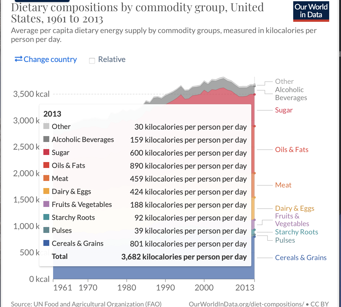
I downloaded American’s diet composition by food groups data from Our World in Data. I selected this data because I’m interested in seeing how the average American’s diet composition has changed from 1961 to 2013.
This is the link to the data.
The following code chunk loads the package I will use to read in and prepare the data for analysis

library(tidyverse)
library(tidyr)

Read the data in

dietary_compositions_by_commodity_group <- read_csv(here::here("_posts/2022-04-27-project-part-1/dietary-compositions-by-commodity-group.csv"))

Use glimpse to see the names and types of the columns

glimpse(dietary_compositions_by_commodity_group)

Rows: 8,154
Columns: 13
$ Entity                                                                <chr> …
$ Code                                                                  <chr> …
$ Year                                                                  <dbl> …
$ `Other (FAO (2017)) (kilocalories per person per day)`                <dbl> …
$ `Sugar (FAO (2017)) (kilocalories per person per day)`                <dbl> …
$ `Oils & Fats (FAO (2017)) (kilocalories per person per day)`          <dbl> …
$ `Meat (FAO (2017)) (kilocalories per person per day)`                 <dbl> …
$ `Dairy & Eggs (FAO (2017)) (kilocalories per person per day)`         <dbl> …
$ `Fruit and Vegetables (FAO (2017)) (kilocalories per person per day)` <dbl> …
$ `Starchy Roots (FAO (2017)) (kilocalories per person per day)`        <dbl> …
$ `Pulses (FAO (2017)) (kilocalories per person per day)`               <dbl> …
$ `Cereals and Grains (FAO (2017)) (kilocalories per person per day)`   <dbl> …
$ `Alcoholic Beverages (FAO (2017)) (kilocalories per person per day)`  <dbl> …

Use output from glimpse (and View) to prepare the data for analysis

Create the object food_group that is a list of food groups I want to extract from the dataset
Change the name of 3rd column to Year and the 5th column to Sugar_Calories
Use filter to extract the rows that I want to keep: Entity = “United States”, Year >= 1961
Select the columns to keep: Entity, Year, Sugar_Calories
Assign the output to usa_diet
Display the first 10 rows of usa_diet

regions  <- c("United States")


usa_diet  <- dietary_compositions_by_commodity_group  %>% 
  rename(Year = 3, `Other` = 4, `Sugar`= 5, `Oils & Fats` = 6, `Meats` = 7, `Dairy & Eggs` = 8, `Fruit and Vegetables` = 9, `Starchy Roots` = 10, `Pulses` = 11, `Cereals and Grains` = 12, `Alcoholic Beverages` = 13) %>%
  filter( Year >= 1961, Entity %in% regions)  %>% 
  select(Entity, Year, Other, Sugar, `Oils & Fats`, Meats, `Dairy & Eggs`, `Fruit and Vegetables`, `Starchy Roots`, Pulses, `Cereals and Grains`, `Alcoholic Beverages`)  

usa_diet

# A tibble: 53 × 12
   Entity         Year Other Sugar `Oils & Fats` Meats `Dairy & Eggs`
   <chr>         <dbl> <dbl> <dbl>         <dbl> <dbl>          <dbl>
 1 United States  1961    21   515           532   355            450
 2 United States  1962    21   520           526   359            439
 3 United States  1963    23   509           534   368            440
 4 United States  1964    22   525           558   377            447
 5 United States  1965    24   533           553   367            450
 6 United States  1966    24   533           560   380            453
 7 United States  1967    25   544           569   393            439
 8 United States  1968    25   549           577   402            438
 9 United States  1969    23   562           593   386            437
10 United States  1970    24   566           611   388            438
# … with 43 more rows, and 5 more variables:
#   `Fruit and Vegetables` <dbl>, `Starchy Roots` <dbl>,
#   Pulses <dbl>, `Cereals and Grains` <dbl>,
#   `Alcoholic Beverages` <dbl>

Check that the avg total calories for sugar in 2013 equals the total in the graph

usa_diet  %>% filter(Year == 2013)  %>% 
  summarise(total_sugarcals = sum(`Sugar`))

# A tibble: 1 × 1
  total_sugarcals
            <dbl>
1             600

Format the original data set to make it easier to plot. Condense the values of columns 3 : 12 under a single row using the function pivot_longerfrom the Tidyrpackage and then assign output to usa_diet2. Display usa_diet2.

usa_diet2 <- pivot_longer(usa_diet, cols = 3:12, names_to = "Food Group", values_to = "Calories") %>% 
  select(Year, "Food Group", Calories )

usa_diet2

# A tibble: 530 × 3
    Year `Food Group`         Calories
   <dbl> <chr>                   <dbl>
 1  1961 Other                      21
 2  1961 Sugar                     515
 3  1961 Oils & Fats               532
 4  1961 Meats                     355
 5  1961 Dairy & Eggs              450
 6  1961 Fruit and Vegetables      144
 7  1961 Starchy Roots              90
 8  1961 Pulses                     36
 9  1961 Cereals and Grains        628
10  1961 Alcoholic Beverages       109
# … with 520 more rows

Add a picture.

See how to change the width in the R Markdown Cookbook

Write the data to file in the project directory

write_csv(usa_diet2, file="usa_diet2.csv")